Traffic flow is the study of interactions between travelers (including pedestrians, cyclists, drivers, and their vehicles) and infrastructure (including highways, signage, and traffic control devices), with the aim of understanding and developing an optimal transport network with efficient movement of traffic and minimal traffic congestion problems.

Attempts to produce a mathematical theory of traffic flow date back to the 1920s, when Frank Knight first produced an analysis of traffic equilibrium, which was refined into Wardrop’s first and second principles of equilibrium in 1952.The fundamental diagram of traffic flow is a diagram that gives a relation between the traffic flux (vehicles/hour) and the traffic density (vehicles/km). A macroscopic traffic model involving traffic flux, traffic density and velocity forms the basis of the fundamental diagram. It can be used to predict the capability of a road system, or its behaviour when applying inflow regulation or speed limits.

Basic Premises

• There is a connection between traffic density and vehicle velocity: The more vehicles are on a road, the slower their velocity will be.
• To prevent congestion and to keep traffic flow stable, the number of vehicles entering the control zone has to be smaller or equal to the number of vehicles leaving the zone in the same time.
• At a critical traffic density and a corresponding critical velocity the state of flow will change from stable to unstable.
• If one of the vehicles brakes in unstable flow regime the flow will collapse.
  The primary tool for graphically displaying information in the study traffic flow is the fundamental diagram. Fundamental diagrams consist of three different graphs: flow-density, speed-flow, and speed-density. The graphs are two dimensional graphs. All the graphs are related by the equation “flow = speed * density”; this equation is the essential equation in traffic flow. The fundamental diagrams were derived by the plotting of field data points and giving these data points a best fit curve. With the fundamental diagrams researchers can explore the relationship between speed, flow, and density of traffic.

Speed-density

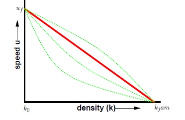
Speed Density Diagram

The speed-density relationship is linear with a negative slope; therefore, as the density increases the speed of the roadway decreases. The line crosses the speed axis, y, at the free flow speed, and the line crosses the density axis, x, at the jam density. Here the speed approaches free flow speed as the density approaches zero. As the density increases, the speed of the vehicles on the roadway decreases. The speed reaches approximately zero when the density equals the jam density.

Flow-density
In the study of traffic flow theory, the flow-density diagram is used to determine the traffic state of a roadway.

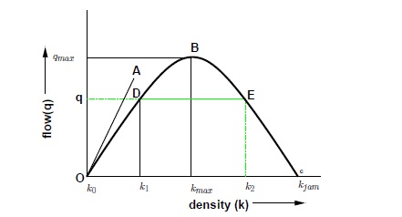
Flow Density Curve

Currently, there are two types of flow density graphs. The first is the parabolic shaped flow-density curve, and the second is the triangular shaped flow-density curve. Academia views the triangular shaped flow-density curve as more the accurate representation of real world events. The triangular shaped curve consists of two vectors. The first vector is the free flow side of the curve. This vector is created by placing the free flow velocity vector of a roadway at the origin of the flow-density graph. The second vector is the congested branch, which is created by placing the vector of the shock wave speed at zero flo

w and jam density. The congested branch has a negative slope, which implies that the higher the density on the congested branch the lower the flow; therefore, even thoug

h there are more cars on the road, the number of cars passing a single point is less than if there were fewer cars on the road. The intersection of free flow and congested vectors is the apex of the curve and is considered the capacity of the roadway, which is the traffic condition at which the maximum number of vehicles can pass by a point in a given time period. The flow and capacity at which this point occurs is the optimum flow and optimum density, respectively. The flow density diagram is used to give the traffic condition of a roadway. With the traffic conditions, time-space diagrams can be created to give travel time, delay, and queue lengths of a road segment.

Speed-flow
Speed – flow diagrams are to determine the speed at which the optimum flow occurs. There are currently two shapes of the speed-flow curve. The speed-flow curve also consists of two branches, the free flow and congested branches.

Source(s):

Wikipedia